Intro
Recently, I am studying The Elements of Statistical Learning out of my own interest. An interesting topic they covered briefly on their online videos is bootstrap. Bootstrap, in the simplest terms, is the process of generating samples from sample. Say you collected a sample of n data points, a bootstrap sample is generated by sampling n data points from the original sample you collected with replacement. (So Given a sample size of n, you are able to generate \(n^n\) bootstrap samples.)
One of the assertion that they made on bootstrap is that bootstrap samples contains, on average, around two thirds of the original data points (Or to be more precise, 63.2%). And in the online video Rob said it is not hard to prove it.
I believed in him and tried to prove it myself, only to find myself still pondering after 2 hours. It turns out that there are (at least) two ways to prove it: an easy way and a hard way. Unfortunately and unintentionally, I realized that I have chosen the hard way to prove it… (An excuse why I couldn’t prove such an “easy” problem).
As an afterthought, I realised I was trying to characterize the entire distribution of the Number of unique data points in a bootstrap sample while I could have simply computed the mean of it (more excuse for myself).
Easy way first
Let \(Y\) be the number of unique data points in a bootstrap sample:
\[Y = \sum_{i = 1}^{n} {I(x_i \in S)}\]
where \(S\) is the original sample, \(x_i\) is the \(i^{th}\) data point in the original sample and n is number of data points in the bootstrap sample (which is also the number of data points in the original sample). Therefore, the expected number of unique data points in a bootstrap sample is:
\[ \begin{align} \mathbb{E} [Y] & = \mathbb{E} \left[\sum_{i = 1}^{n} {I(x_i \in S)}\right] \\ & = \sum_{i = 1}^{n} \mathbb{E} \left[ {I(x_i \in S)}\right] \\ & = \sum_{i = 1}^{n} \mathbb{P} \left( x_i \in S\right) \\ & = n\mathbb{P} \left( x_1 \in S\right) \end{align} \]
What is \(\mathbb{P} \left( x_1 \in S\right)\) ? Well, this is fairly simple if we instead calculate \(\mathbb{P} \left( x_1 \notin S\right)\):
\[ \begin{align} \mathbb{P} \left( x_1 \notin S\right) &= \prod_{i = 1}^{n} \mathbb{P} \left(x^{*}_i \notin S\right) \\ &= \left(1 - \frac{1}{n}\right)^n \end{align} \]
Note that \(x_i^*\) represent the \(i^{th}\) element in the bootstrap sample whereas \(x_i\) represent the \(i^{th}\) element in the original sample. Therefore, the expected number of unique data points in a bootstrap sample, as a proportion of total data points is:
\[ \begin{align} \mathbb{E} \left[\frac{Y}{n}\right] &= \mathbb{P} \left( x_1 \in S\right) \\ &= 1 - \mathbb{P} \left( x_1 \notin S\right) \\ &= 1 - \left( 1 - \frac{1}{n} \right)^n \end{align} \]
So the expected proportion still depends on n, but it converges to \(1 - e^{-1}\) very quickly as n gets large:
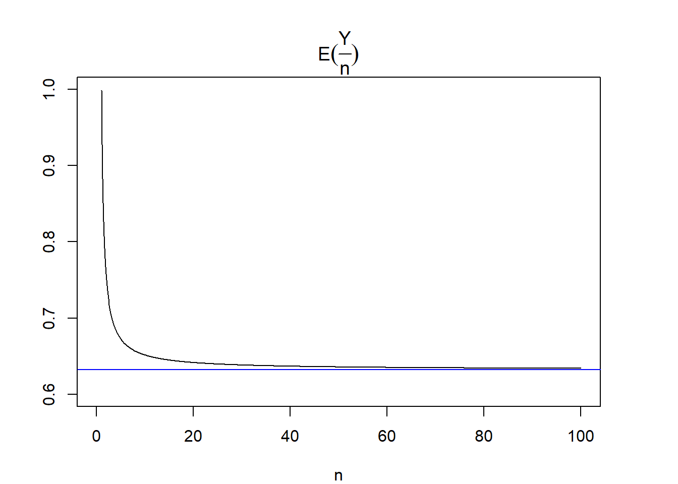
We can see that the expected proportion gets very close to 0.632 when sample size is greater than 20.
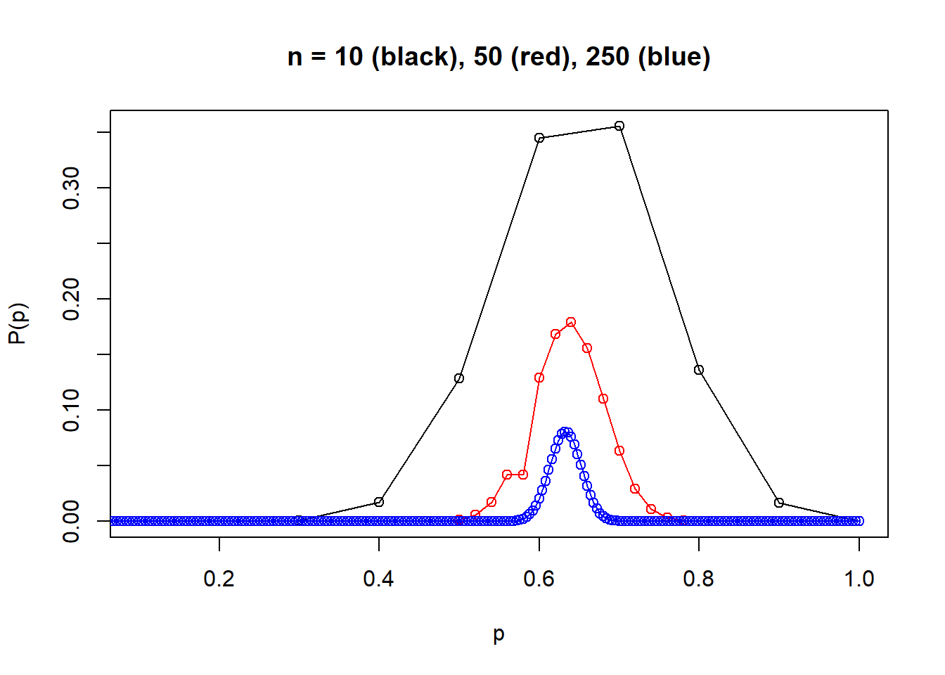
So the easy way is fairly easy. But it only gives you the mean of the distribution. What does the distribution of the proportion of original data points in a bootstrap sample look like?
The hard way
Another way to get to calculate an expected value is to derive the distribution first and then take the expection. It doesn’t sound hard, but it does require me to devote more brain energy. As humans are lazy, I will just come back to it later when I have time (blame human not me). But here’s a paper that solves exactly what I failed to solve.
The paper discusses the distribution of the number of unique original data points in a bootstrap sample, which is simply the distribution of the proportion of unique orignial data points in a bootstrap sample scaled by sample size. Standing on their shoulder, I know the probability of obtaining \(k\) unique original data points is:
\[ \mathbb{P}(k) = \frac{(n)_k}{n^n} { n \brace k } \]
where \(n\) is sample size, \((n)_k = \frac{n!}{(n-k)!}\) is a falling factorial, and \({n \brace k}\) is a Stirling number of the second kind (It basically represents number of ways to partition a set of n objects into k non-empty subsets.). If I denote \(p\) as the the proportion of unique orignial data points in a bootstrap sample (\(p = \frac{k}{n}\)), then:
\[ \begin{align} \mathbb{P}_P(p) &= \mathbb{P}_K(np) \\ &= \frac{(n)_{np}}{n^n} { n \brace np } \\ \end{align} \]
With the help of gmp package, I can visualize this distribution, although it took me some time to grasp bigz and bigq class implemented in gmp package. They are needed because \(n^n\), \((n)_{np}\) and \({n \brace np}\) involves incredibly large integers that can easily exceed the capability of R’s 32 bit integer. \(20^{20} \approx 10^{26}\) which already exceeds maximum integer in R by quite a big margin.
Below is a graph showing the distribution for n = 10, 50 and 250. One can almost imaging that when n gets larger, say 1000, the distribution will basically concentrate on a very narrow range around 0.632. Note some points are wrong because I ran into precision problems and I guess it’s because R loses precision in floating point arithmatics as the numbers involved are too big. I guess I should be able to avoid this by using gmp more properly, but I’ll leave it to the next time.