Intro
With online courses, I feel I am usually too rushed to complete them for at least two reasons:
- Save money because I pay a monthly fee.
- Eager to get a certificate so I can overestimate myself.
So this time I think perhaps I should pause and let it precipitate.
I recently rushed through a Coursera course Neural Networks and Deep Learning. What’s most amazing about this course, in my opinion, is that it teaches you to build a neural network model in python, from ground up. I did a few statistic courses before and I have never needed to write an algorithm from ground up. All I did was calling glm() or some other modelling functions already there and they do the fitting for me. To make sure I internalize the ideas and the algorithm, I am writing this post to implement a neural network in R (I can’t put python source code online as per course requirement.)
Perhaps the most difficult part in this course is to get my head around the different conventions between statistics and computer science. For example, in almost all statistics literature, the data matrix, \(X\), is organized so that it has \(N\) rows and \(p\) columns, where \(N\) is the sample size and p is number of coefficients (or features plus one). In deep learning, it’s the opposite, the data matrix is \(p\) by \(N\), \(p\) rows, \(N\) columns. Some other nitty-gritty details: sample size is represented by \(m\) rather than \(N\), number of features by \(n_x\) rather than \(p\), etc. It’s these little things that caused a somewhat big cognitive barrier initially. Here I decided to follow the traditional statistics convention, just to make sure I really internalize the idea rather than the formula.
Data Preparation
I am using the same datasets that were used in the online course, which you can find them here.
library(h5)
library(dplyr)
library(imager)
library(tidyr)
library(ggplot2)
library(stringr)

train_set_orig <- h5file("../../static/datasets/train_catvnoncat.h5")
test_set_orig <- h5file("../../static/datasets/test_catvnoncat.h5")

train_set_x_orig <- readDataSet(train_set_orig["train_set_x"])
train_set_y <- readDataSet(train_set_orig["train_set_y"])
test_set_x_orig <- readDataSet(test_set_orig["test_set_x"])
test_set_y <- readDataSet(test_set_orig["test_set_y"])
The training set contains 209 images of cats and non-cats and the test set contains 50 images. Each image is 64 pixels wide, 64 pixels high, and 3 color channels.
With imager package, plotting is a such a pleasing thing to do. Let’s take a look at the first five images and the dimensions of the datasets:
train_set_plot <- as.cimg(aperm(train_set_x_orig, perm = c(3, 2, 1, 4)))

train_set_y[1:6]
## [1] 0 0 1 0 0 0par(mfrow = c(2, 3), mai = c(0,0,0.2,0))
for (i in 1:6) plot(train_set_plot, i, main = paste0("image ", i), axes = FALSE)
str(train_set_x_orig)
##  int [1:209, 1:64, 1:64, 1:3] 17 196 82 1 9 84 56 19 63 23 ...
str(train_set_y)
##  num [1:209] 0 0 1 0 0 0 0 1 0 0 ...
str(test_set_x_orig)
##  int [1:50, 1:64, 1:64, 1:3] 158 115 255 254 96 26 239 236 19 231 ...
str(test_set_y)
##  num [1:50] 1 1 1 1 1 0 1 1 1 1 ...
Next let’s reshape the data so it’s ready for modelling - we need to flatten the image so that each image can be represented by a vector of dimension \(64 \times 64 \times3 = 12288\). Again, I am following traditional statistics convention, adding a leading 1 to this vector which represents the intercept, so each observation is \(p = 12288 + 1 = 12289\) dimensional. After the reshaping, the training set train_set_x is 209 by 12289 and the leading column of train_set_x is a column of 1 representing the intercept. Similarly the test_set_x is 50 by 12289. I use aperm to keep data preparation result identical to that of python.
train_set_x_flatten <- aperm(train_set_x_orig, c(1, 4, 3, 2))
dim(train_set_x_flatten) <- c(209, 64 * 64 * 3)
train_set_x <- cbind(1, train_set_x_flatten/255)
dim(train_set_x)
## [1] 209 12289test_set_x_flatten <- aperm(test_set_x_orig, c(1, 4, 3, 2))
dim(test_set_x_flatten) <- c(50, 64 * 64 * 3)
test_set_x <- cbind(1, test_set_x_flatten/255)
dim(test_set_x)## [1] 50 12289Logistic Regression
The implementation of the optimization of the logistic regression, from a neural network’s perspective, is organized into three procedures:
- Forward propagation
- This involves calculating the predictions and cost based on current weights (coefficients).
- Backward propagation.
- This involves calculating the gradient which gives the direction in which the cost function has the steepest slope.
- Gradient descent
- This involves updating the weights (coefficients) using the gradients and learn rate.
These three procedures are repeated many times to minimize the cost function. In spirit, this is identical to maximizing the likelihood function.
The online course used computaional graph to reason about the algorithm and organize the computation. The computational graph breaks down the optimization process into smaller pieces like a divide-and-conquer strategy. It also helps one to think about what intermediate values need to be cached to improve the efficiency of the algorithm. However, I wanted to have just a few equations here so I don’t need to hold too many things in my really small working memory.
Again I will be following traditional statistics notations (adapted from The Elements of Statisitcal Learning): all vectors are column vectors denoted by non-bold lower case letters (e.g. \(w\)), except when a vector has N (sample size) components in which case it is denoted by bold lower case letters (\(\mathbf{a}\)). Elements of a vector can be accessed via subscript (e.g. \(w_j\) represent the \(j^{th}\) element of \(w\)). Matrices are denoted by capital letters (e.g. \(X\)) and elements can be accessed by \(X_{ij}\). Again, the reason for this is that I want to make sure I internalize the algorithm and a good way for doing this is to show that I can reproduce the algorithm with a different set of notations. Also this set of convention is probably more friendly to R.
Forward Propagation
Now suppose the 209 data points are a simple random sample, so the joint probability distribution is simply the product of individual probability distributions, so does the joint likelihood function. Let’s start from individual data points. For the \(i^{th}\) data point, the likelihood \(L_i\) can be written as:
\[ \begin{align} L_i(w, b) & = \mathbf{p}_i^{\mathbf{y}_i}(1 - \mathbf{p}_i)^{(1 - \mathbf{y}_i)} \\ & = \mathbf{a}_i^{\mathbf{y}_i}(1 - \mathbf{a}_i)^{(1 - \mathbf{y}_i)} \end{align} \]
Where
\[ \mathbf{a}_i = \mathbf{p}_i = \sigma(\mathbf{z}_i) = \sigma(x_i^T w + b) \]
In the above two equations, \(\mathbf{a}_i = \mathbf{p}_i\) is the \(i^{th}\) component of the activation (N-)vector, or the true probability of being a cat for the \(i^{th}\) example. \(\mathbf{z}_i\) is the linear predictor for the \(i^{th}\) example (the \(i^{th}\) component of the N-vector \(\mathbf{z}\)), \(w\) is a p-vector (p here means number of features) representing slope coefficients (a.k.a weights in deep learning), \(b\) is the intercept coefficient (a.k.a bias), \(x_i\) is a p-vector representing the observations of all features of \(i^{th}\) example.
Note here an interesting fact about sigmoid function which is that it’s derivative can be written as a function of the sigmoid function itself in a fairly simple form, it is this property that ends up cancelling many terms so that the slope can be calculated efficiently:
\[ \begin{align} \frac{d\mathbf{a}_i}{d\mathbf{z}_i} & = \frac{d\sigma(\mathbf{z}_i)}{d\mathbf{z}_i} \\ & = \frac{d}{d\mathbf{z}_i} \left( \frac{1}{1 + e^{-\mathbf{z}_i}} \right) \\ & = \frac{-1}{(1 + e^{-\mathbf{z}_i})^2} e^{-\mathbf{z}_i} (-1) \\ & = \frac{e^{-\mathbf{z}_i}}{(1 + e^{-\mathbf{z}_i})^2} \\ & = \frac{1}{1 + e^{-\mathbf{z}_i}} \frac{e^{-\mathbf{z}_i}}{1 + e^{-\mathbf{z}_i}} \\ & = \mathbf{a}_i (1 - \mathbf{a}_i) \end{align} \]
This will be useful in backward propagation.
If we consider all data points, we can write down a similar equation but encompass all data points. Here, I am actually going to redefine weights \(w\) and data matrix \(X\): include \(b\) into \(w\) (i.e. \(w_1 = b\)) and augment \(X\) with a column of 1s as it’s first column (so the new \(X\) is \(N\) by \((p + 1)\) and the new \(w\) is a (p + 1)-vector). This results in a more elegant equation, hence less corner cases to consider when implementing the algorithm.
\[ \mathbf{a} = \mathbf{p} = \sigma(\mathbf{z}) = \sigma(\mathbf{X} w) \]
where \(\mathbf{a} = \mathbf{p}\) is a N-vector representing activations or the true probabilities of being a cat for each example. \(\mathbf{z}\) is the linear predictor.
Similarly, the likelihood, \(L(w)\), and log likelihood, \(l(w)\), for all data points can be written as
\[ L(w) = \prod_{i = 1}^N \left( \mathbf{a}_i^{\mathbf{y}_i}(1 - \mathbf{a}_i)^{(1 - \mathbf{y}_i)} \right) \]
and
\[ \begin{align} l(w) & = log\left( \prod_{i = 1}^N \left( \mathbf{a}_i^{\mathbf{y}_i}(1 - \mathbf{a}_i)^{(1 - \mathbf{y}_i)} \right) \right) \\ & = \sum_{i = 1}^N \left( \mathbf{y}_i log(\mathbf{a}_i) + (1 - \mathbf{y}_i) log(1 - \mathbf{a}_i) \right) \\ & = \mathbf{y}^T log(\mathbf{a}) + (\mathbf{1} - \mathbf{y})^T log(\mathbf{1} - \mathbf{a}) \end{align} \]
In deep learning, people usually use cost function as a measure of how well the estimated function fits to the data. The cost function is simply the negative of the log likelihood divided by the sample size:
\[ J(w) = - \frac{1}{N} \left( \mathbf{y}^T log(\mathbf{a}) + (\mathbf{1} - \mathbf{y})^T log(\mathbf{1} - \mathbf{a}) \right) \]
Backward Propagation
The backward propagation is usually the hardest part in neural networks. It’s especially hard if you want to use proper matrix calculus to derive the equation. Fortunately, the course steps through the derivation in such a way that even you don’t know matrix algebra, you are able to arrive at the same equation. All that requires is basic matrix multiplication and scalar calculus. I tried to derive the same result using matrix calculus but no luck in getting there. If you do, do let me know!
Anyway, here’s a more non-mathematician friendly way. Let
\[ C_i = - \mathbf{y}_i log(\mathbf{a}_i) - (1 - \mathbf{y}_i) log(1 - \mathbf{a}_i) \]
denote the cross entropy for the \(i^{th}\) data point, which is simple the negative of the log likelihood for that data point (Note that \(\mathbf{y}_i\) and \(\mathbf{a}_i\) are both scalar). Therefore
\[ J(w) = \frac{1}{N}\sum_{i = 1}^{N} C_i \]
For the \(i^{th}\) data point and the \(j^{th}\) weight, we have:
\[ \begin{align} \frac{dC_i}{dw_{j}} & = \frac{dC_i}{d\mathbf{a}_i} \frac{d\mathbf{a}_i}{d\mathbf{z}_i} \frac{d\mathbf{z}_i}{dw_{j}}\\ & = \left( - \frac{\mathbf{y}_i}{\mathbf{a}_i} + \frac{1 - \mathbf{y}_i}{1 - \mathbf{a}_i} \right) \mathbf{a}_i (1 - \mathbf{a}_i) x_{ij} \\ & = (\mathbf{a}_i - \mathbf{y}_i) x_{ij} \end{align} \]
Generalize the above equation to the cost function \(J\) with matrix notation, we have:
\[ \begin{align} \frac{dJ}{dw_{j}} & = \frac{1}{N}\sum_{i = 1}^{N} \frac{dC_i}{dw_j} \\ & = \frac{1}{N} \sum_{i = 1}^{N} \left( (\mathbf{a}_i - \mathbf{y}_i) x_{ij} \right) \\ & = \frac{1}{N} (\mathbf{a} - \mathbf{y})^T \mathbf{x}_j \end{align} \]
And further generalize the above equation to all weights:
\[ \begin{align} \frac{dJ}{dw} & = \begin{bmatrix} \frac{dJ}{dw_1} \\ \frac{dJ}{dw2} \\ . \\ .\\ .\\ \frac{dJ}{dw_p} \end{bmatrix} \\ & = \frac{1}{N} \begin{bmatrix} (\mathbf{a} - \mathbf{y})^T \mathbf{x}_1 \\ (\mathbf{a} - \mathbf{y})^T \mathbf{x}_2 \\ . \\ .\\ .\\ (\mathbf{a} - \mathbf{y})^T \mathbf{x}_3 \end{bmatrix} \\ & = \frac{1}{N} \begin{bmatrix} (\mathbf{a} - \mathbf{y})^T \mathbf{x}_1 & (\mathbf{a} - \mathbf{y})^T \mathbf{x}_2 & ... & (\mathbf{a} - \mathbf{y})^T \mathbf{x}_3 \end{bmatrix}^T \\ & = \frac{1}{N} \left((\mathbf{a} - \mathbf{y})^T X \right)^T \\ & = \frac{1}{N} X^T (\mathbf{a} - \mathbf{y}) \end{align} \]
So, that’s all the math that’s required. I tried to write down those equations in matrix or vector notation because being able to write down an equation in matrix form means being able to take advantage of vectorization. As a side note, given that there is no scalar in R, it feels that vectorization comes as a free lunch!
Implementation
The equations are the key, implementation is really straight forward once we have the equations written down in matrix notation. The logic is simple:
we initialize weights, say initialize to zeros;
do a forward propagation, i.e., calculating the predictions and cost based on the current weights;
do a backward propagation, i.e. calculating the gradients;
update the weights by moving them down the steepest slope. A better-known term for this is: Gradient descent;
repeat the step 2 - 4 a lot of times until the algorithm converges or stop early as a sort of “regularization” (prevent over fitting).
Let’s modularize the above steps so the code is cleaner and hopefully reusable:
- define a helper function, sigmoid, which is the term in deep learning for inverse logit function:
sigmoid <- function(x) {
  1 / (1 + exp(-x))
}- forward propagation function (so easy!)
forward_propagation <- function(X, w, activation = sigmoid) {
  activation(X %*% w)
}- compute cost (still easy)
compute_cost <- function(y, a, N = length(y)) {
  -(1 / N) * (sum(y * log(a)) + sum((1 - y) * log(1 - a)))
}- backward propagation function (can’t be easier)
backward_propagation <- function(X, y, a, N = length(y)) {
  (1/N) * crossprod(X, a - y)
}- update weights (should I write this as a function?)
update_grads <- function(w, dw, learn_rate) {
  w - learn_rate * dw
}
Having written down the above functions, let’s compose them together. The function below may seem a little messy, but that’s because I am basically recording all intermediate results for every single iteration, so that I can better understand what the algorithm is doing.
- Model function
logistic_model <- function(X, y, X_test, y_test, learn_rate, iter) {

  # sample size and number of features
  N <- nrow(X)
  N_test <- nrow(X_test)
  p <- ncol(X)

  # initialize weights
  w <- matrix(NA, nrow = iter + 1, ncol = p)
  w[1, ] <- 0

  # initialize dw as a matrix to record gradients from every iteration
  dw <- matrix(NA, nrow = iter, ncol = p)

  # initialize activations, predictions, accuracy rates for training set
  a_train <- matrix(NA, nrow = iter, ncol = N)
  pred_train <- matrix(NA, nrow = iter, ncol = N)
  accuracy_train <- numeric(iter)

  # initialize activations, predictions, accuracy rates for test set
  a_test <- matrix(NA, nrow = iter, ncol = N_test)
  pred_test <- matrix(NA, nrow = iter, ncol = N_test)
  accuracy_test <- numeric(iter)

  # initialize cost
  J <- numeric(iter)


  # main iterations
  for (i in 1:iter) {

    # forward propagation to get current activations, predictions
    # and accuracy rate for both train and test
    a_train[i, ] <- forward_propagation(X, w[i, ])
    pred_train[i, ] <- ifelse(a_train[i, ] > 0.5, 1, 0)
    accuracy_train[i] <- mean(pred_train[i, ] == y)

    a_test[i, ] <- forward_propagation(X_test, w[i, ])
    pred_test[i, ] <- ifelse(a_test[i, ] > 0.5, 1, 0)
    accuracy_test[i] <- mean(pred_test[i, ] == y_test)

    # compute cost for the current iteration
    J[i] <- compute_cost(y, a_train[i, ], N = N)

    # backward propagation to get gradients
    dw[i, ] <- backward_propagation(X, y, a_train[i, ], N = N)

    # update gradients (gradient descent)
    w[i + 1, ] <- update_grads(w[i, ], dw[i, ], learn_rate = learn_rate)

  }

  list(a_train = a_train,
       a_test = a_test,
       pred_train = pred_train,
       pred_test = pred_test,
       accuracy_train = accuracy_train,
       accuracy_test = accuracy_test,
       J = J,
       dw = dw,
       w = w)
}
Train Model
Learning rate is perhaps the single most important hyperparameters in this simple model. Let’s train the model with learning rates 0.0005, 0.005, 0.05 and 0.5 for 2000 iterations:
lr_0005 <- logistic_model(X = train_set_x, y = train_set_y, X_test = test_set_x, y_test = test_set_y, learn_rate = 0.0005, iter = 2000)

lr_005 <- logistic_model(X = train_set_x, y = train_set_y, X_test = test_set_x, y_test = test_set_y, learn_rate = 0.005, iter = 2000)

lr_05 <- logistic_model(X = train_set_x, y = train_set_y, X_test = test_set_x, y_test = test_set_y, learn_rate = 0.05, iter = 2000)

lr_5 <- logistic_model(X = train_set_x, y = train_set_y, X_test = test_set_x, y_test = test_set_y, learn_rate = 0.5, iter = 2000)
Understand the Result
As mentioned above, the whole purpose of this exercise is to better understand what the algorithm is doing, so let’s examine the results in detail. First, let’s check the evolution of the cost function:
par(mfrow = c(2,2))
plot(lr_0005$J, type = "l", lwd = 1, col = "green", ylim = 0:1,
     xlab = "iteration", ylab = "cost", main = "Learn rate = 0.0005")
plot(lr_005$J, type = "l", lwd = 1, col = "orange", ylim = 0:1,
     xlab = "iteration", ylab = "cost", main = "Learn rate = 0.005")
plot(lr_05$J, type = "l", lwd = 1, col = "red",
     xlab = "iteration", ylab = "cost", main = "Learn rate = 0.05")
plot(lr_5$J, type = "l", lwd = 1, col = "black",
     xlab = "iteration", ylab = "cost", main = "Learn rate = 0.5")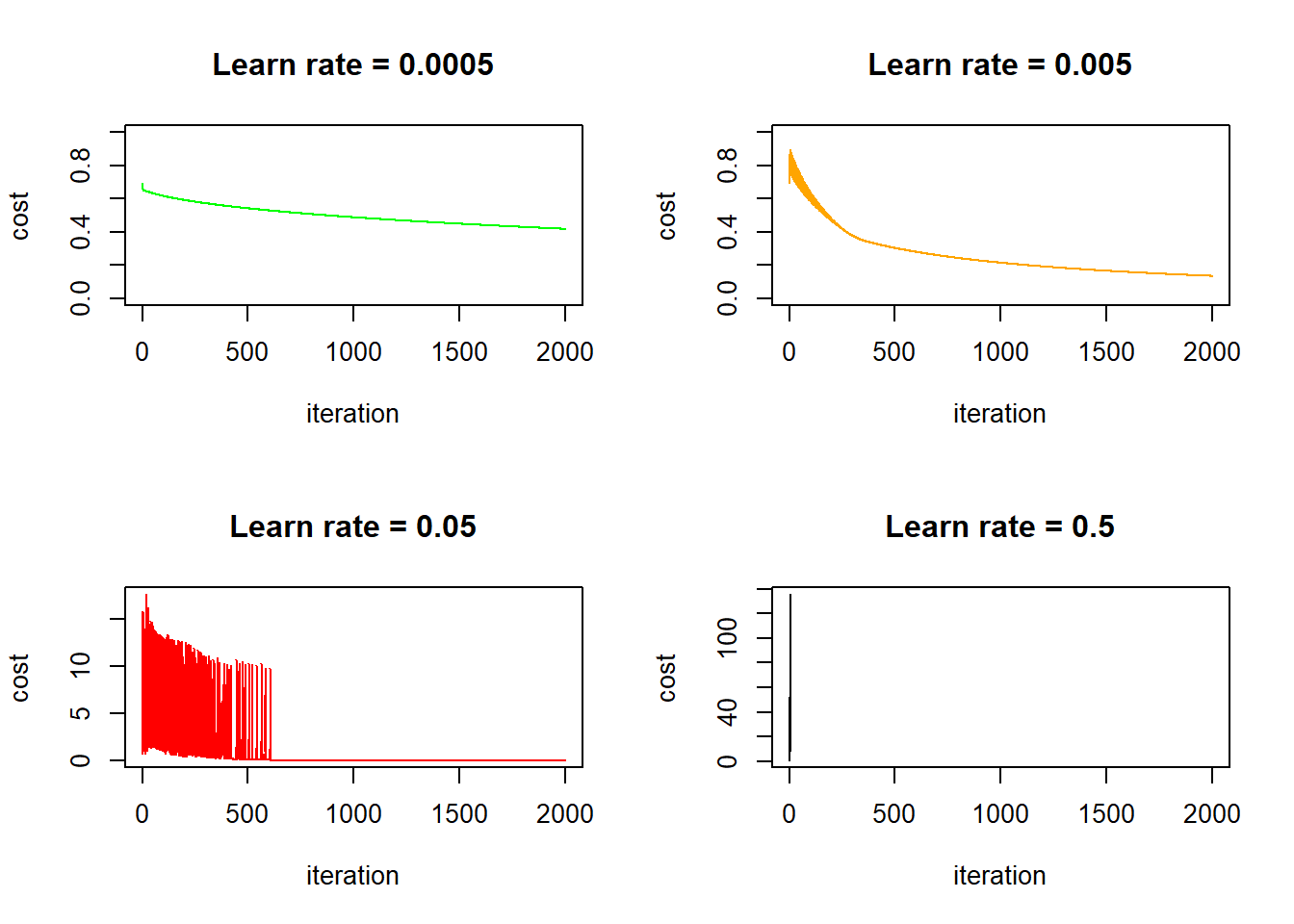
This is interesting, in the first three cases (learn rate = 0.0005, 0.005, 0.05) the cost function eventually goes down, but for the two cases where learn rates equal to 0.005 and 0.05, the cost initially bumps up and down quite dramatically. I think this is because the learn rate is too big - the gradient descent strides too big steps and it’s stepping over the optimal point back and forth initially, until it luckily hits a point where the gradient is very close to zero and it no longer stride large steps. Take away? Always check the cost/iteration graph to make sure that your cost stabilize eventually! In fact, the online course used the learn rate of 0.005, which corresponds to the second plot above. It oscillates a little bit initially but stabilizes quickly after less than 500 iterations. It’s not a bad choice: selecting a lower learn rate (say 0.0005) means your algorithm takes longer to get to the same cost, on the other hand, selecting a higher learn rate (say 0.5, the bottom right graph) means you risk numerical issues (explained later). Also worth noting is that in this particular case, if we keep iterating with a sensible learn rate, we will eventually end up with a perfect fit because we have more features than data points.
Cost function is mainly a function of activations, so it must be that the activations are causing the cost function to jump up and down. Let’s check how activations, the estimated probabilities of being a cat, evolves. Since plotting all 209 data points is just a mess, I am plotting the first 50 training examples:
par(mfrow = c(2, 2))
matplot(lr_0005$a_train[, 1:50], type = "l", lty = 1, xlab = "Iteration", ylab = "Activation", main = "learn rate = 0.0005")
matplot(lr_005$a_train[, 1:50], type = "l", lty = 1, xlab = "Iteration", ylab = "Activation", main = "learn rate = 0.005")
matplot(lr_05$a_train[, 1:50], type = "l", lty = 1, xlab = "Iteration", ylab = "Activation", main = "learn rate = 0.05")
matplot(lr_5$a_train[, 1:50], type = "l", lty = 1, xlab = "Iteration", ylab = "Activation", main = "learn rate = 0.5")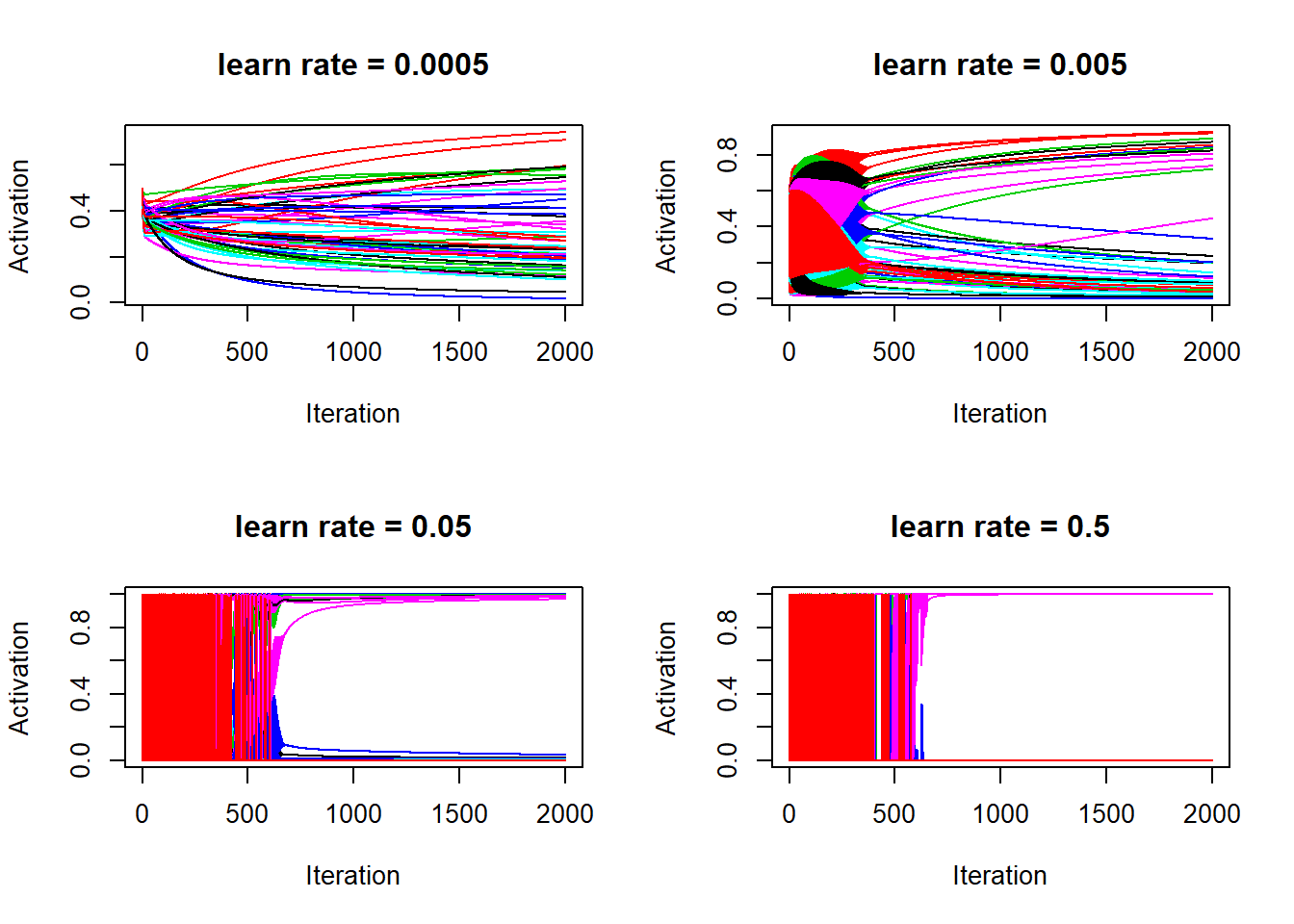
So the above four graphs are the evidence that activations are the culprit for causing the cost function to jump up and down. Also, it’s clear that with higher learn rate, activations (or the estimated probabilities for being a cat) quickly converges to either 1 or 0. It’s over fitting, for learn rate = 0.5, after 2000 iterations, the activations are basically identical to the training labels:
range(lr_5$a_train[2000, ] - train_set_y)## [1] -0.001764490 0.006920968In fact, for learn rate = 0.5, some activations are so close to 1 that 1 - a is so close to zero that R thinks log(1 - a) is NaN, hence the cost cannot be properly computed and the cost evolution for learn rate = 0.5 is not showing properly.
Activation is a function of weights, so it must be that the weights jumps up and down initially for large learn rates. let’s check how the weights evolves. For simplicity, I am just displaying a random sample 10 weights from the 12289 weights:
par(mfrow = c(2, 2))
set.seed(123)
sample_weights <- sample(12289, 10)
matplot(lr_0005$w[, sample_weights], type = "l", lty = 1, lwd = 1, xlab = "Iteration", ylab = "weights", main = "Learn rate = 0.0005")
matplot(lr_005$w[, sample_weights], type = "l",  lty = 1,lwd = 1, xlab = "Iteration", ylab = "weights", main = "Learn rate = 0.005")
matplot(lr_05$w[, sample_weights], type = "l", lty = 1, lwd = 1, xlab = "Iteration", ylab = "weights", main = "Learn rate = 0.05")
matplot(lr_5$w[, sample_weights], type = "l", lty = 1, lwd = 1, xlab = "Iteration", ylab = "weights", main = "Learn rate = 0.5")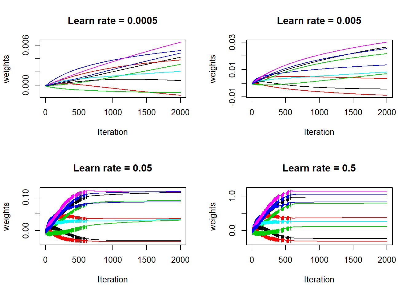
Yes, the weights were not stable for large learn rates: the gradient descent takes too big steps so for a particular weight, it is stepping back and forth, until is slowing moves towards a more flat region. Next, check the evolution of accuracy on both train and test sets:
par(mfrow = c(2, 2))
plot(lr_0005$accuracy_train, type = "l", col = "red", ylim = c(0, 1),
     xlab = "Iteration", ylab = "Accuracy rate", main = "learn rate = 0.0005")
lines(lr_0005$accuracy_test, type = "l", col = "green")
plot(lr_005$accuracy_train, type = "l", col = "red", ylim = c(0, 1),
     xlab = "Iteration", ylab = "Accuracy rate", main = "learn rate = 0.005")
lines(lr_005$accuracy_test, type = "l", col = "green")
plot(lr_05$accuracy_train, type = "l", col = "red", ylim = c(0, 1),
     xlab = "Iteration", ylab = "Accuracy rate", main = "learn rate = 0.05")
lines(lr_05$accuracy_test, type = "l", col = "green")
plot(lr_5$accuracy_train, type = "l", col = "red", ylim = c(0, 1),
     xlab = "Iteration", ylab = "Accuracy rate", main = "learn rate = 0.5")
lines(lr_5$accuracy_test, type = "l", col = "green")
legend("bottomright", col = c("red", "green"), lty = 1, legend = c("train", "test"))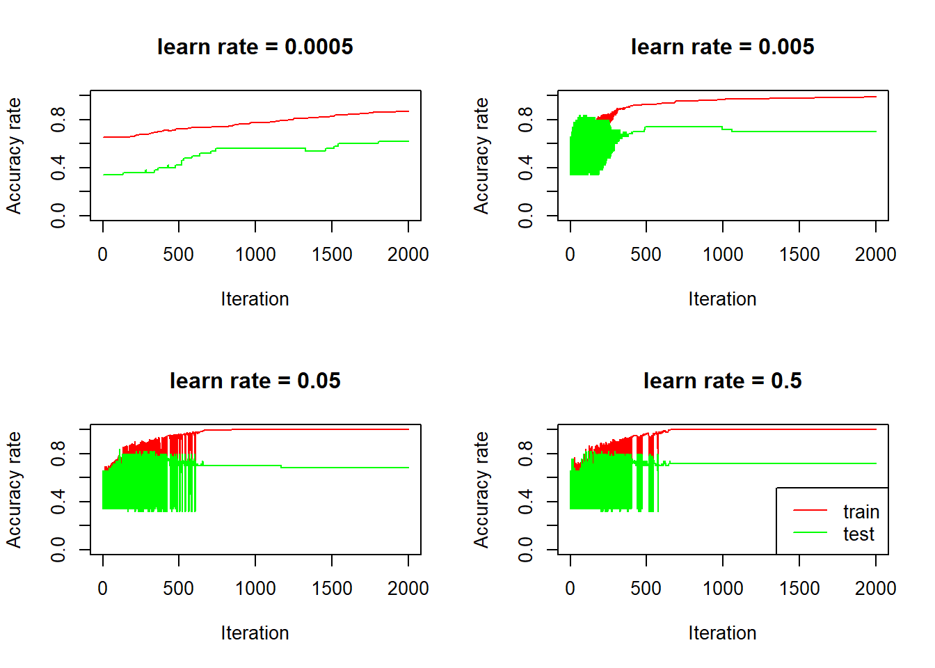
Again, we see that for bigger learn rates, the accuracy rates are quite volatile, on both train and test set, initially (learn rate is so big that for each iteration, the activations goes up and down by a large amount), and the accuracy rate on the test set seems to be going down after it stabilizes, over fitting in action.
For the model with smallest learn rate (0.0005), the accuracy rate on the test set goes up steadily, it starts at 0.34, which is the proportion of non cat in the test set:
mean(test_set_y == 0)## [1] 0.34This is expected because we initialized weights to be all zeros, which means the activations for the first pass are \(\mathbf{a}_i = \sigma(x_i^Tw_i) = \sigma(X_i^T0) = \frac{1}{1 + e^{-0}} = 0.5\). Since 0.5 is not greater than 0.5, the predictions are basically all 0s.
It turns out that learn rate equal to 0.005 gives best performance out of the three learn rates: The test performance stabilizes to 0.68, reaching more than 70% if stopping early. Note that the null model (predicting cats no matter what) actually gives 66% accuracy on this test set. So it’s not a big improvement and we need more test examples to make firmer conclusions.
we can also check the how false positive rate (non-cat being incorrectly classified as cat) and false negative rate evolves (cat being incorrectly classified as non-cat), for both train and test sets:
fp_and_fn <- function(model) {
  main <- deparse(substitute(model))
  fp_train <- rowMeans(model$pred_train[, train_set_y == 0])
  fn_train <- 1 - rowMeans(model$pred_train[, train_set_y == 1])
  fp_test <- rowMeans(model$pred_test[, test_set_y == 0])
  fn_test <- 1 - rowMeans(model$pred_test[, test_set_y == 1])

  plot(fp_train, type = "l", col = "red", ylim = 0:1, ylab = "Error rate",
       main = paste0(main, " train"))
  lines(fn_train, col = "green")
  plot(fp_test, type = "l", col = "red", ylim = 0:1, ylab = "",
       main = paste0(main, " test"))
  lines(fn_test, col = "green")
}

par(mfrow = c(4, 2), mai = c(0.25,0.5,0.25,0))
fp_and_fn(lr_0005); fp_and_fn(lr_005); fp_and_fn(lr_05); fp_and_fn(lr_5)
legend("topright", col = c("red", "green"), legend = c("False positive", "False negative"), lty = 1, cex = 0.8)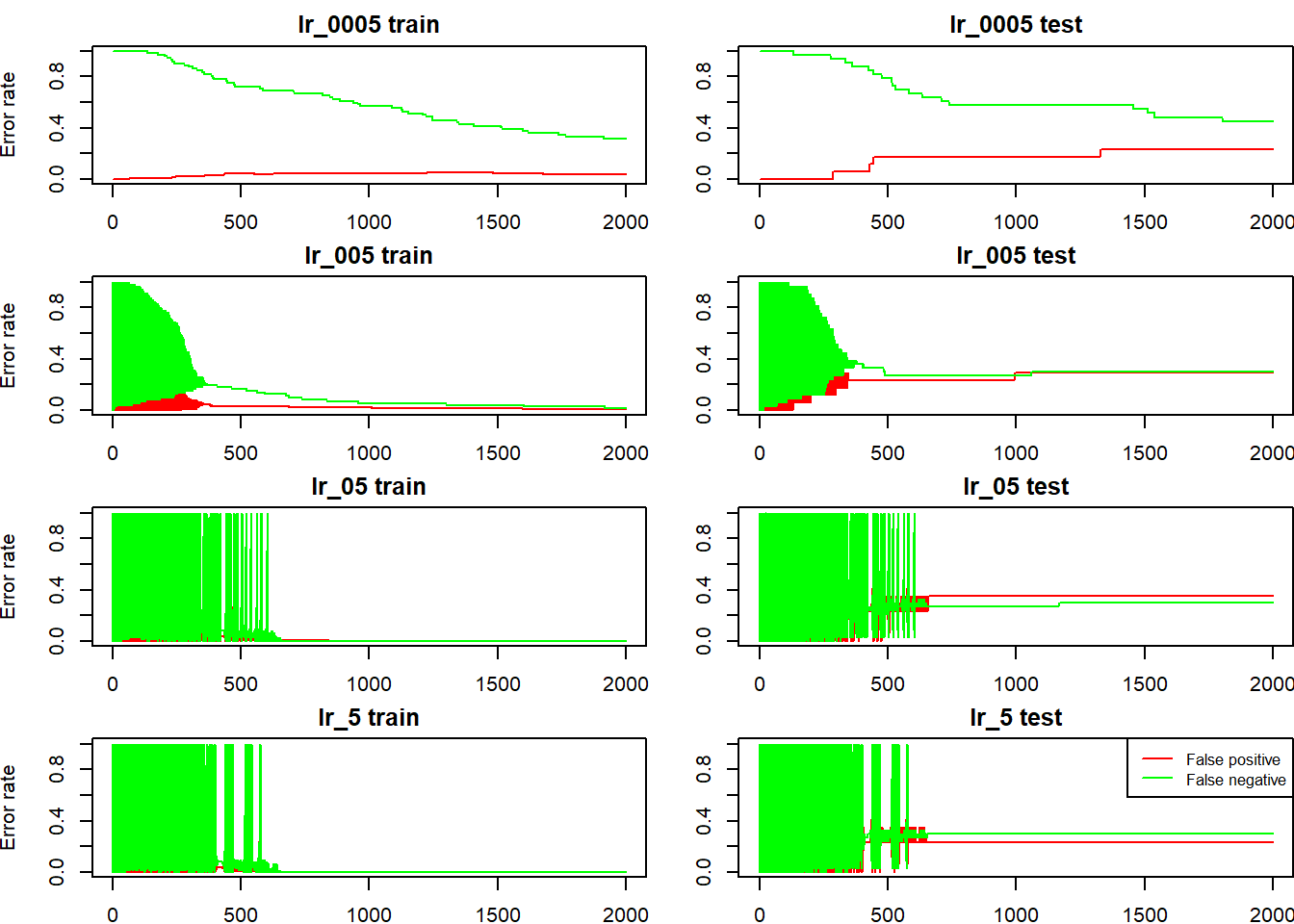
Finally, let’s check how the predictions evolves. I am only doing this on the test set. First define a helper function that plots both predictions and activations:
model_evolution <- function(model, alpha = 1) {
  p <- model$a_test %>%
    as.data.frame() %>%
    setNames(paste0("V", str_pad(1:50, width = 2, pad = 0), ": ", if_else(test_set_y == 1, "cat", "non-cat"))) %>%
    mutate(Iteration = 1:2000) %>%
    gather(key = "Example", value = "Activation", -Iteration) %>%
    left_join(
      model$pred_test %>%
        as.data.frame() %>%
        setNames(paste0("V", str_pad(1:50, width = 2, pad = 0), ": ", if_else(test_set_y == 1, "cat", "non-cat"))) %>%
        mutate(Iteration = 1:2000) %>%
        gather(key = "Example", value = "Prediction", -Iteration),
      by = c("Example", "Iteration")

    ) %>%
    gather(key = "outcome", value = "value", Activation, Prediction) %>%
    # mutate(Example = factor(Example, levels = paste0("V", 1:50, sep = ""))) %>%
    ggplot(aes(Iteration, value, group = outcome, color = outcome)) +
    geom_line(alpha = alpha) +
    facet_wrap(facets = ~Example, nrow = 10, ncol = 5) +
    theme_void() +
    theme(strip.background = element_blank(),
          strip.switch.pad.grid = unit(0, "cm"),
          strip.text.x = element_text(size = 8),
          panel.background = element_rect(fill = "white", colour = "grey50"),
          panel.border = element_rect(fill = NA, color = "black"),
          axis.text = element_blank(),
          axis.ticks = element_blank()
          )

  print(p)
}- For learn rate equal to 0.0005
model_evolution(lr_0005) 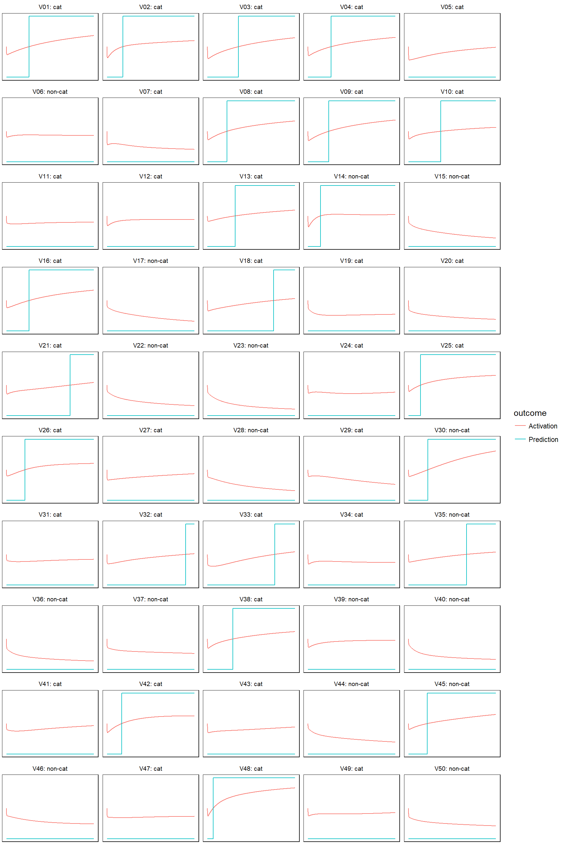
- learn rate = 0.005
model_evolution(lr_005, 0.5)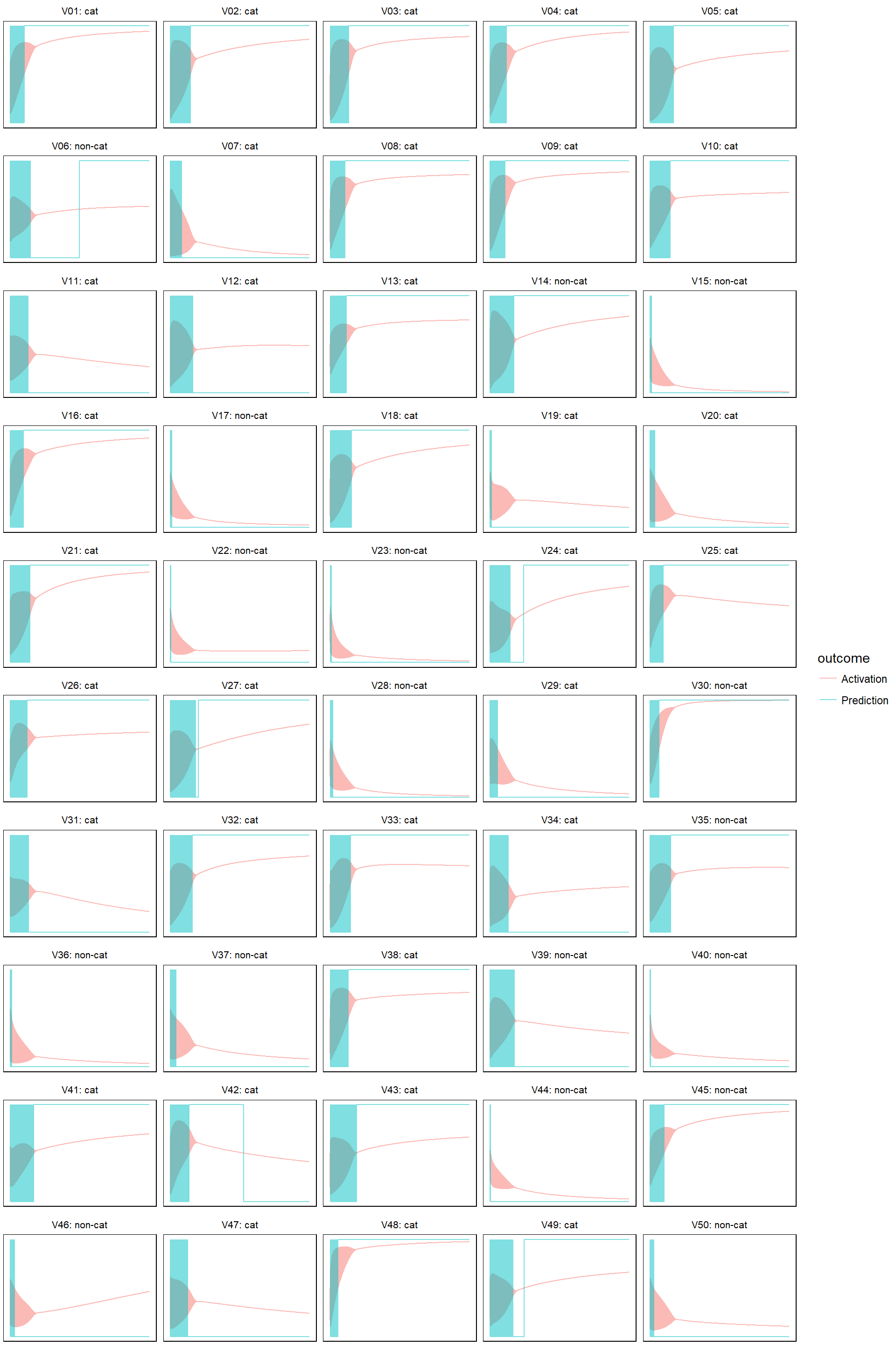
- learn rate 0.05
model_evolution(lr_05, 0.5)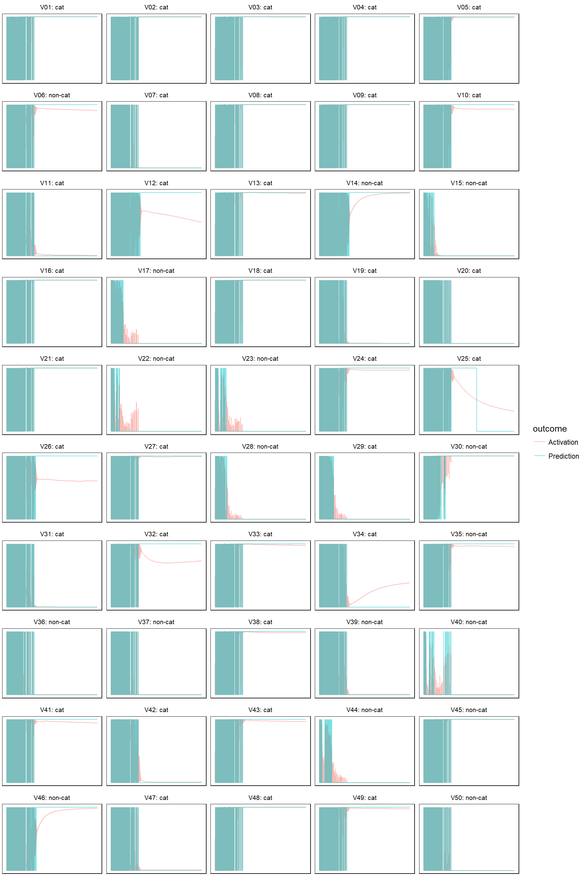
- learn rate 0.5
model_evolution(lr_5, 0.5)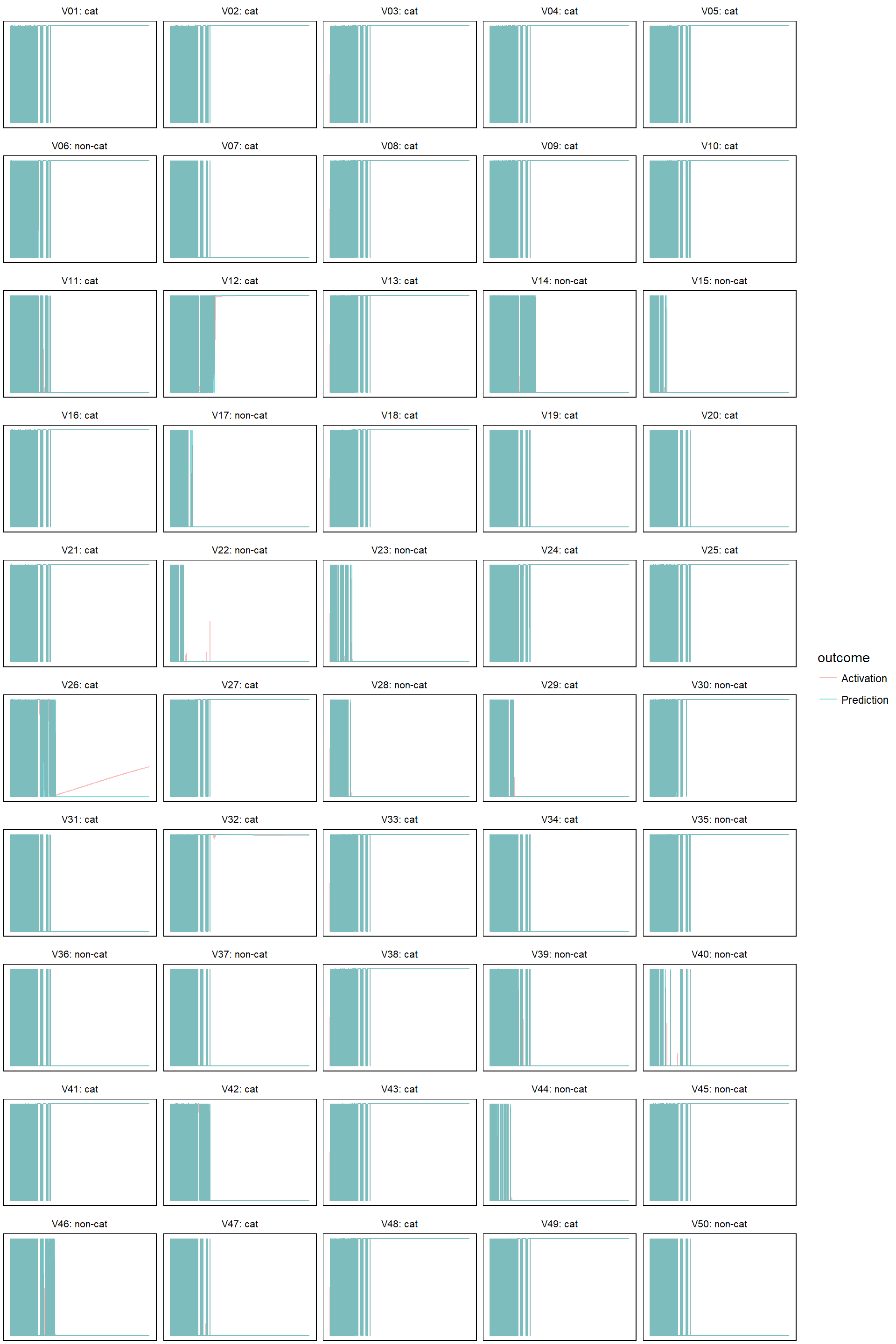
Summary
It feels pretty satisfactory to write the algorithm from scratch and implement it using nothing but base R code. Although I should realize that this is simply doing what all those great packages doing, in a much more clumsy way. But, sometimes, you don’t really understand until you do it yourself.